EEGlass

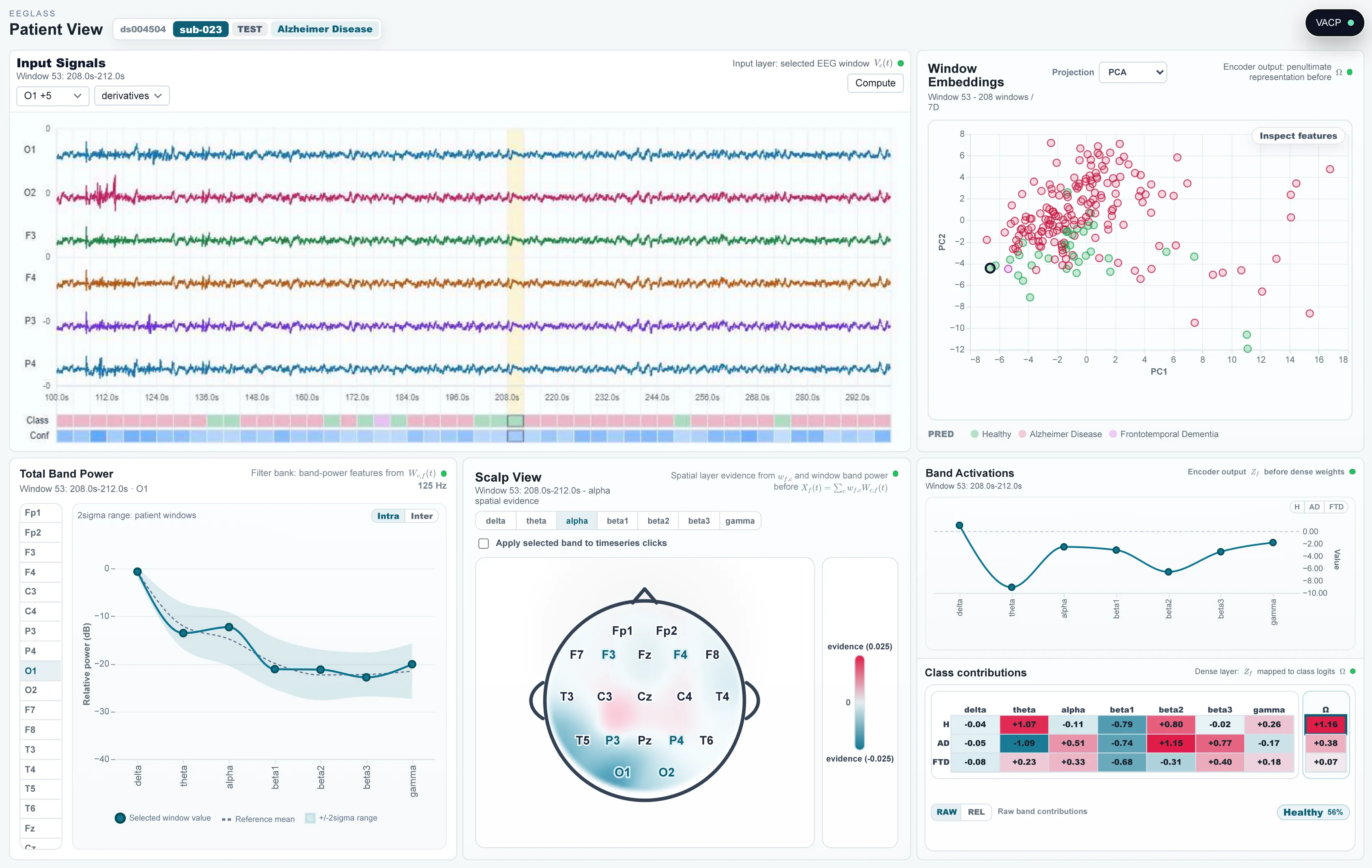
To make clinical diagnoses more understandable, we present a visual interactive dashboard on top of the efficient xEEG classifier network architecture, which puts a special emphasis on explainibility of the model and outcome. This dataset and model focusses on Alzheimer’s Disease (AD) and Frontotemporal Dementia (FTD), every step in the classification is presented in a visual and understandable way, on top of an integrated EEG database viewer.

EEGlass

To make clinical diagnoses more understandable, we present EEGlass, a visual interactive dashboard on top of the efficient xEEGNet classifier network architecture, which puts a special emphasis on explainability of the model and outcome. This dataset and model focuses on Alzheimer’s Disease (AD) and Frontotemporal Dementia (FTD); every step in the classification is presented in a visual and understandable way, on top of an integrated Electroencephalography (EEG) database viewer.

EEGlass Preview

The Model

xEEGNet is a fully interpretable classifier with only $F \cdot (C + L + 2) = 168$ trainable parameters. For a subject $k$ : $C = 19$ channels $V_c(t)$ , $N = L \cdot f_s = 500$ samples ( $L = 4$ s, $f_s = 125$ Hz).

1. Bandpass filters ( $F = 7$ fixed FIR filters $\delta, \theta, \alpha, \beta_1, \beta_2, \beta_3, \gamma$ ):

$W_{c,f}(t) = \mathrm{Filter}_f\left[V_c(t)\right]$

2. Spatial mixing with learned weights $w_{c,f}$ :

$X_f(t) = \sum_{c=1}^{C} w_{c,f} W_{c,f}(t)$

3. Batch norm + band power (square, average, log):

$\hat{Z}_f = 10 \log_{10}\left(\frac{1}{N_1} \sum_{i=0}^{N_1 - 1} X_f(t_i)^2\right)$

4. Linear classifier ( $M \in \mathbb{R}^{L \times F}$ , $L = 3$ classes):

$\mathbf{\Omega} = M \hat{\mathbf{Z}} \in \mathbb{R}^{L}, \qquad \mathbf{y} = \arg\max(\mathbf{\Omega})$

$M_{l,f} \hat{Z}_f$ gives the signed per-band class contribution shown in the dashboard.

In short: fixed bandpass filters $\rightarrow$ learned spatial mixing $\rightarrow$ bandpower $\rightarrow$ linear classifier. Every intermediate value has a direct physical meaning, so clinicians inspect architecture-intrinsic evidence rather than post-hoc saliency maps.

Supported Dimensionality Reductions

PCA, t-SNE and UMAP projections, selectable in all embedding views (PCA is the default).

Example Use-Case

As an example workflow, a user can start with a new participant by selecting a typical point in the window embedding (R2) to see the predicted output. The Total Band Power panel immediately shows how typical this window's band powers are for the patient, and whether the (e.g. alpha) bands align more with the healthy or AD/FTD cohort (R3). The Scalp View and Band Activations panel make explicit which channels and bands drove the prediction (R1).

Inspecting the raw signal, the user can judge for themselves whether the window looks atypical, where, for each patient and time window individually, the topomap, band activations, and total band power panel indicate which channels and bandpowers are worth a closer look (the corresponding bandpass filter can also be applied to the time-series view), directing the user to the most interesting aspects and making comparison easy while keeping them in control.

Contribute

Combination of all frontend and backend utilities, and baseline for xEEG dashboard development.

To install dependencies:

uv install
bun install

If uv version is newer, use:

uv sync

To start a development server:

uv run fastapi dev backend/app.py --reload-dir backend/
bun dev

To format code:

ruff format
prettier -w .

Also useful: ruff check --fix --unsafe-fixes.

Docker Deployment

Build and start the full stack:

docker compose up --build

The compose setup starts three services:

dataset-downloader: downloads and extracts the configured dataset into the datasets Docker volume, then exits.
backend: starts only after dataset-downloader completed successfully. It serves the API on http://localhost:8000.
frontend: serves the UI on http://localhost:3000.

The default dataset is large. docker-compose.yml also contains a commented smaller dataset URL (only 5 patients instead of 88) that can be swapped into DATASET_URL to test the download flow without downloading the full 4.2 GB dataset.